Bottom-up Parsing

Bottom-Up Parsing Process

Bottom-up parsing is the process of reducing an input string to the start symbol S of the grammar. At each reduction step, a specific substring matching the body of a production (RHS) is replaced by the nonterminal at the head of that production (LHS). The key decisions during bottom-up parsing are about when to reduce and about what production to apply, as the parse proceeds.

Handle Pruning

• Bottom-up parsing during a left-to-right scan of the input constructs a right-most derivation in reverse.
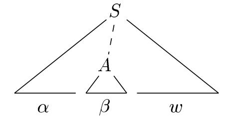
• A "handle" is a substring that matches the body of a production, and whose reduction represents one step along the reverse of a rightmost derivation.
• A handle A → β in the parse tree for w:

Shift-Reduce Parsing

• Shift-reduce parsing is a form of bottom-up parsing in which a stack holds grammar symbols and an input buffer holds the rest of the string to be parsed.
• Primary operations are shift and reduce.
• During a left-to-right scan of the input string, the parser shifts zero or more input symbols onto the stack, until it is ready to reduce a string of grammar symbols on top of the stack.
• It then reduces to the head of the appropriate production with number R_x.
• The parser repeats this cycle until it has detected an error or until the stack contains the start symbol and the input is empty.
• There are actually four possible actions a shift-reduce parser can make:
• Shift. Shift the next input symbol onto the top of the stack.
• Reduce. The right end of the string to be reduced must be at the top of the stack. Locate the left end of the string within the stack and decide with what nonterminal to replace the string.
• Accept. Announce successful completion of parsing.
• Error. Discover a syntax error and call an error recovery routine

Primary operations

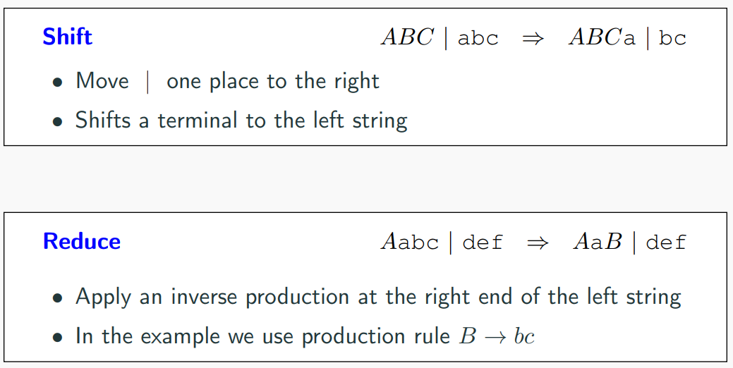
Shift-Reduce Parsing Notations

• We use $ to mark the bottom of the stack and also the right end of the input.
• Split string into two substrings, right and left, the dividing point is marked by a |.
• Right substring is still not examined by parser (a string of terminals).
• Left substring has both terminals and non-terminals.
• Note: The | is not part of the string
• Initially, all input is unexamined " | a1a2...an$".

Shift-Reduce Parsing Example

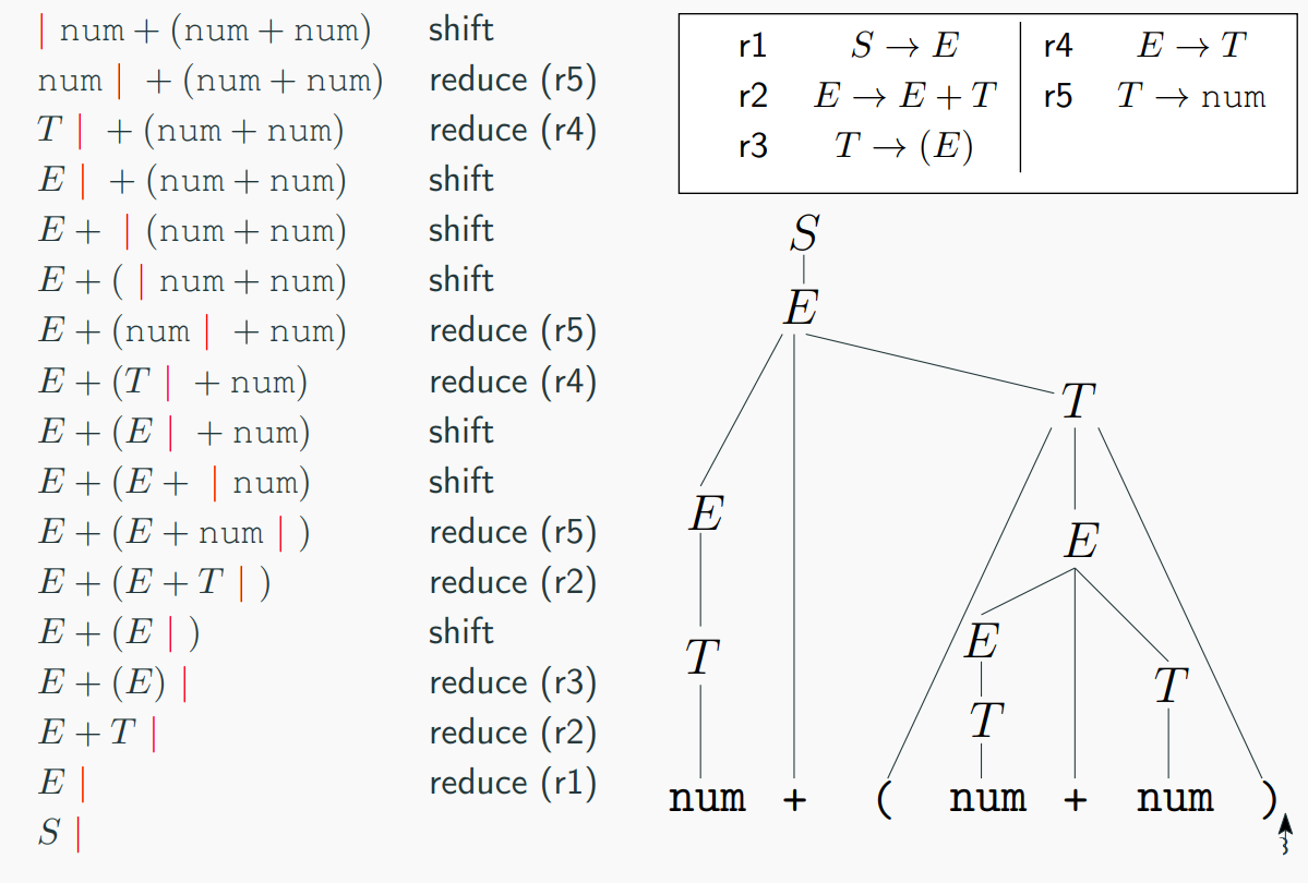
Let's consider the following productions:

r1  S->E 
r4  E->T
r2 E ->E+T 
r3  T->(E)
r5  T ->num

And the input string |num+(num+num)$. The parsing process would go as follows:

|num+(num+num)     shift
num|+(num+num)   reduce(r5)   
T|+(num+num)    reduce(r4)
E|+(num+num)  shift
E+|(num+num)   shift
E+(|num+num)   shift
E+(num|+num)  reduce(r5)
E+(T|+num)   reduce(r4)
E+(E|+num)   shift
E+(E+|num)   shift
E+((E+num|)   reduce(r5)
E+(E+T|)    reduce(r2)
E+(E|)   shift
E+(E)    reduce(r3)
E+T    reduce(r2)
E|    reduce(r1)
S|

Here, shift means pushing the next input symbol onto the top of the stack, and reduce means popping zero or more symbols off the stack (production RHS) and pushing a non-terminal on the stack (production LHS)

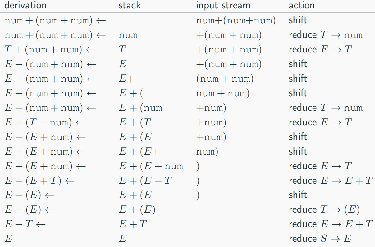
Shift-Reduce Parsing Stack

• Left substring can be implemented by a stack.
• Top of the stack is the | symbol.
• Shift pushes a terminal on the stack.
• Reduce pops Zero or more symbols of the stack (production RHS) and pushes a non-terminal on the stack (production LHS).

example

Conflicts During Shift-Reduce Parsing

• There are context-free grammars for which shift-reduce parsing cannot be used.

• Every shift-reduce parser for such a grammar can reach a configuration in which the parser, knowing the entire stack and also the next k input symbols, cannot decide:

• Whether to shift or to reduce (a shift/reduce conflict)

• Or cannot decide which of several reductions to make (a reduce/reduce conflict)

• Consider the following ambiguous grammar for if-then-else statements:

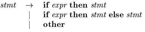
• If we have a shift-reduce parser in configuration:

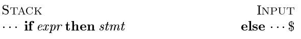
• There is a shift/reduce conflict,
• We cannot tell whether if expr then stmt is the handle.

example - Consider the following productions involving procedure calls and array references: - If we have a shift-reduce parser in configuration: - There is a reduce/reduce conflict, - It is evident that the id on top of the stack must be reduced, but by which production? - The correct choice is production (5) if id is a procedure, but production (7) if id is an array. - We need a precise mechanism to decide which action to take: shift or reduce, if reduce should be taken then to which production?

Final Thoughts

Remember, mastering these concepts takes time and practice. Don't hesitate to ask questions or seek clarification if something is unclear. Happy studying!

LR Parsing and LR Grammars

• LR parsing is the most prevalent type of bottom-up parser today. The term "LR" stands for left-to-right scanning of the input and constructing a rightmost derivation in reverse.
• A grammar for which we can construct a parsing table using an LR parsing algorithm is said to be an LR grammar. The class of grammars that can be parsed using LR methods is a proper superset of the class of grammars that can be parsed with predictive or LL methods.

LR(k) Parsers and Grammars

The "k" in LR(k) refers to the number of input symbols of lookahead that are used in making parsing decisions. The cases where k = 0 or k = 1 are of practical interest. When (k) is omitted, k is assumed to be 1. LR parsers are table-driven, similar to nonrecursive LL parsers.
For a grammar to be LL(k), we must be able to recognize the use of a production by seeing only the first k symbols of what its right side derives.

For a grammar to be LR(k), we must be able to recognize the occurrence of the right side of a production in a right-sentential form, with k input symbols of lookahead. This requirement is far less stringent than the one for LL(k) grammars. The principal drawback of the LR method is that it is too much work to construct an LR parser by hand for a typical programming-language grammar. A specialized tool, an LR parser generator, is needed.

• The most prevalent type of bottom-up parser today is based
• the "R"is for constructing a rightmost derivation in reverse,
• the "k"for the number of input symbols of lookahead that are used in making parsing decisions.
• The cases k = 0 or k = 1 are of practical interest.
• When (k) is omitted, k is assumed to be 1.
• LR parsers are table-driven, much like the non-recursive LL parsers.

Variants of LR Parsers

There are several variants of LR parsers: SLR parsers, LALR parsers, canonical LR(1) parsers, minimal LR(1) parsers, and generalized LR parsers (GLR parsers). LR parsers can be generated by a parser generator from a formal grammar defining the syntax of the language to be parsed. They are widely used for the processing of computer languages. An LR parser reads input text from left to right without backing up and produces a rightmost derivation in reverse. The name "LR" is often followed by a numeric qualifier, as in "LR(1)" or sometimes "LR(k)". To avoid backtracking or guessing, the LR parser is allowed to peek ahead at k lookahead input symbols before deciding how to parse earlier symbols. Typically k is 1 and is not mentioned.

LR(0) parsing

Representing Item Sets

In the context of LR(0) parsing, an item set represents the current state of the parser. Each item in the set corresponds to a production in the grammar, with a dot indicating the current position in the production. For example, if we have a production A -> BC, there will be four items corresponding to this production:

• A -> .BC
• A -> B.C
• A -> BC.
• A -> B.C.

These items represent the different stages of recognizing the production A -> BC.

Closure and Goto of Item Sets

The closure operation takes a set of items and produces a new set containing all items that can be derived from the original set. This is done through a series of steps:

1. Add every item in the original set to the closure set.
2. For each item in the closure set that is of the form A -> α.Bβ, check if there is a production B -> γ in the grammar. If so, add the item B -> .γβ to the closure set.
3. Repeat step 2 until no more new items can be added to the closure set.

The closure ensures that all nonterminals following the dot are expanded into their possible productions, allowing the parser to anticipate all valid next steps. This is a key step in constructing the LR(0) automaton.

The GOTO operation, on the other hand, is used to determine the next state based on the current state and the next input symbol. It is defined as the closure of the set of all items of the form A -> αB.β, where A -> α.Bβ is in the current state.

Intuitively, the GOTO functionis used to define the transitions in the LR(0) automaton for a grammar. The states of the automaton correspond to sets of items, and GOTO(I;B) specifies the transition from the state for I under input B.

Note: Note: By convention, S ′ → S$ is the kernel of the first item, I0. example:

Let's consider a simple grammar:

E -> E + T | T
T -> F | (E)
F -> id

We start with the initial state I0 = {E -> .E + T}. We apply the closure operation to get the closure of I0:

I0 = {E -> .E + T, E -> E + .T}

Then, we apply the GOTO operation with the input symbol E to get the next state:

GOTO(I0, E) = {E -> E + .T, E -> .T}

We continue this process until we reach the final state, which indicates that the input string is valid according to the grammar.

example:

(0) E
′ → E$
(1) E → E + T
(2) E → T
(3) T → T * F
(4) T → F
(5) F → (E)
(6) F → id

CLOSURE(I0 ={︀[E′ → .E$]}︀):

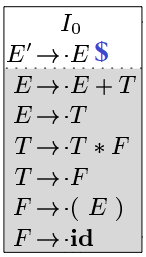
• Start with $[E' \rightarrow \cdot E\$]$.
• For $E$ after the dot, add all $E$-productions: $[E \rightarrow \cdot E + T]$, $[E \rightarrow \cdot T]$.
• For $T$ in $[E \rightarrow \cdot T]$, add all $T$-productions: $[T \rightarrow \cdot T * F]$, $[T \rightarrow \cdot F]$.
• For $F$ in $[T \rightarrow \cdot F]$, add all $F$-productions: $[F \rightarrow \cdot (E)]$, $[F \rightarrow \cdot id]$.
• Repeat until no new items are added, resulting in the full set.

GOTO(I0, E):

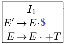
• Take all items in $I_0$ and move the dot past $E$ where $E$ is after the dot.
• From $[E' \rightarrow \cdot E\$]$, move to $[E' \rightarrow E \cdot \$]$.
• From $[E \rightarrow \cdot E + T]$, move to $[E \rightarrow E \cdot + T]$.
• Collect these into $I_1$, excluding items where the dot cannot move past $E$.

Canonical Collection of Sets of LR(0) Items

To construct the parsing table, we need to compute the canonical collection of sets of LR(0) items for an augmented grammar. This involves creating a set of states, where each state represents a set of items. The transitions between states are determined by the GOTO operations.

Algorithm

The items(G') algorithm is like building a map of all the possible steps a parser can take to understand a grammar $ G' $ with an added start rule. Here's how it works in a more natural way:

1. Kick Things Off: It starts by creating a small group called $ C $ with just one set, which is the "closure" of the rule $[S' \rightarrow \cdot S]$, where $ S' $ is a special starting point we add to the grammar.

2. Explore Step by Step: It keeps going through each group of rules (or "sets") in $ C $. For every group and every symbol (like a letter or word) in the grammar:

3. If moving the parser's focus past that symbol (using $ \text{GOTO} $) creates a new, useful set of rules that isn’t already in $ C $, it adds that new set to the group.

4. Keep Going Until Done: It repeats this exploration until no new groups pop up after a full round, meaning we’ve mapped out all the possible parsing states.

example:

Let's consider a slightly more complex grammar:

S -> CC
C -> aC | d

We start by augmenting the grammar to handle left recursion:

(0) S′ → S$
(1) S → CC
(2) C → aC
(3) C → d

The canonical collection in this LR(0) parsing table is computed step by step as follows, based on the given grammar with productions $ S' \rightarrow SS $, $ S \rightarrow CC $, $ C \rightarrow aC $, and $ C \rightarrow d $. The process involves computing closures and GOTO transitions to build the set of states (I0 to I6):

1. Initialize with Closure of Start Symbol:

2. Start with $ I_0 = \text{CLOSURE}([S' \rightarrow \cdot SS]) $.

3. Add $[S' \rightarrow \cdot SS]$.
4. Since $ S $ follows the dot, add all $ S $-productions: $[S \rightarrow \cdot CC]$.
5. Since $ C $ follows the dot in $[S \rightarrow \cdot CC]$, add all $ C $-productions: $[C \rightarrow \cdot aC]$, $[C \rightarrow \cdot d]$.

6. Result: $ I_0 = { [S' \rightarrow \cdot SS], [S \rightarrow \cdot CC], [C \rightarrow \cdot aC], [C \rightarrow \cdot d] } $.

7. Compute GOTO for $ I_0 $:

8. GOTO($ I_0, S $): Move dot past $ S $ in $[S' \rightarrow \cdot SS]$ to get $[S' \rightarrow S \cdot S]$. No further closure needed. Result: $ I_4 $.

9. GOTO($ I_0, C $): Move dot past $ C $ in $[S \rightarrow \cdot CC]$ to get $[S \rightarrow C \cdot C]$. Add $ C $-productions for the second $ C $: $[C \rightarrow \cdot aC]$, $[C \rightarrow \cdot d]$. Result: $ I_3 $.
10. GOTO($ I_0, a $): Move dot past $ a $ in $[C \rightarrow \cdot aC]$ to get $[C \rightarrow a \cdot C]$. Add $ C $-productions: $[C \rightarrow \cdot aC]$, $[C \rightarrow \cdot d]$. Result: $ I_2 $.

11. GOTO($ I_0, d $): Move dot past $ d $ in $[C \rightarrow \cdot d]$ to get $[C \rightarrow d \cdot]$. This is a reduce item. Result: $ I_1 $.

12. Expand from New States:

13. GOTO($ I_3, C $): Move dot past second $ C $ in $[S \rightarrow C \cdot C]$ to get $[S \rightarrow CC \cdot]$. This is a reduce item. Result: $ I_6 $.

14. GOTO($ I_2, C $): Move dot past $ C $ in $[C \rightarrow a \cdot C]$ to get $[C \rightarrow aC \cdot]$. This is a reduce item. Result: $ I_5 $.

15. GOTO($ I_4, $ $): Move dot past $ S $ in $[S' \rightarrow S \cdot S]$ with end marker $ $ $ to get $[S' \rightarrow SS \cdot]$. This is an accept state. Result: Accept (no new state needed).

16. Iterate Until No New States:

17. Check all new states ($ I_1, I_2, I_3, I_4, I_5, I_6 $) for further GOTO transitions.

18. $ I_1, I_5, I_6 $ are reduce states with no further moves.
19. $ I_2 $ and $ I_3 $ were already expanded.
20. No new states are generated, so the collection is complete: $ { I_0, I_1, I_2, I_3, I_4, I_5, I_6 } $.

The resulting states and transitions form the canonical collection, with actions (shift, reduce, accept) assigned based on the dot positions and grammar rules.

Structure of the LR Parsing Table

The LR parsing table consists of two parts: a parsing-action function ACTION and a goto function GOTO. The ACTION function determines what action the parser should take based on the current state and the next input symbol. The GOTO function determines the next state based on the current state and the next input symbol.

example
Assume that we have these:

(0) S′ → S$
(1) S → CC
(2) C → aC
(3) C → d

Now let's construct the LR(0) parsing table: 1. Prepare the Framework: - Create a grid with rows labeled by states 0 through 6 (matching the canonical collection states I0 to I6). - Divide the columns into two sections: "Action" for terminals ($ a $, $ d $, $ $ $) and "Goto" for nonterminals ($ S $, $ C $). - Initialize all cells as empty, ready to be filled based on the state items and transitions. 2. Analyze Each State for Actions:

• State 0 ($ I_0 = { [S' \rightarrow \cdot SS], [S \rightarrow \cdot CC], [C \rightarrow \cdot aC], [C \rightarrow \cdot d] } $):

  • $ [C \rightarrow \cdot aC] $: $ \text{GOTO}(I_0, a) = I_2 $, so set Action[$ a $] = "S2" (shift to 2).
  • $ [C \rightarrow \cdot d] $: $ \text{GOTO}(I_0, d) = I_1 $, so set Action[$ d $] = "S1" (shift to 1).
  • No complete items or $ $ $-related moves, so Action[$ $ $] = "err" (error).
  • State 1 ($ I_1 = { [C \rightarrow d \cdot] } $):
  • $ [C \rightarrow d \cdot] $ is a complete item, reduce by $ C \rightarrow d $ (assume $ R_3 $), so set Action[$ a $] = "R3", Action[$ d $] = "R3", Action[$ $ $] = "R3".

  • State 2 ($ I_2 = { [C \rightarrow a \cdot C], [C \rightarrow \cdot aC], [C \rightarrow \cdot d] } $):

  • $ [C \rightarrow \cdot aC] $: $ \text{GOTO}(I_2, a) = I_2 $, so set Action[$ a $] = "S2" (shift to 2).

  • $ [C \rightarrow \cdot d] $: $ \text{GOTO}(I_2, d) = I_1 $, so set Action[$ d $] = "S1" (shift to 1).
  • No complete items or $ $ $-moves, so Action[$ $ $] = "err".

  • State 3 ($ I_3 = { [S \rightarrow C \cdot C], [C \rightarrow \cdot aC], [C \rightarrow \cdot d] } $):

  • $ [C \rightarrow \cdot aC] $: $ \text{GOTO}(I_3, a) = I_2 $, so set Action[$ a $] = "S2" (shift to 2).

  • $ [C \rightarrow \cdot d] $: $ \text{GOTO}(I_3, d) = I_1 $, so set Action[$ d $] = "S1" (shift to 1).
  • No complete items or $ $ $-moves, so Action[$ $ $] = "err".

  • State 4 ($ I_4 = { [S' \rightarrow S \cdot S] } $):

  • No terminals to shift on, and $[S' \rightarrow S \cdot S]$ with $ $ $ completes the parse, so set Action[$ $ $] = "accept".

  • No valid moves for $ a $ or $ d $, so Action[$ a $] = "err", Action[$ d $] = "err".

  • State 5 ($ I_5 = { [C \rightarrow aC \cdot] } $):

  • $ [C \rightarrow aC \cdot] $ is a complete item, reduce by $ C \rightarrow aC $ (assume $ R_2 $), so set Action[$ a $] = "R2", Action[$ d $] = "R2", Action[$ $ $] = "R2".

  • State 6 ($ I_6 = { [S \rightarrow CC \cdot] } $):

  • $ [S \rightarrow CC \cdot] $ is a complete item, reduce by $ S \rightarrow CC $ (assume $ R_1 $), so set Action[$ a $] = "R1", Action[$ d $] = "R1", Action[$ $ $] = "R1".

• Analyze Each State for Gotos:

• State 0:
  • $ \text{GOTO}(I_0, S) = I_4 $, so set Goto[$ S $] = 4.
  • $ \text{GOTO}(I_0, C) = I_3 $, so set Goto[$ C $] = 3.
• State 1: No nonterminal transitions, so Goto[$ S $] and Goto[$ C $] remain empty.
• State 2:
  • $ \text{GOTO}(I_2, C) = I_5 $, so set Goto[$ C $] = 5.
• State 3:
  • $ \text{GOTO}(I_3, C) = I_6 $, so set Goto[$ C $] = 6.
• States 4, 5, 6: No further nonterminal transitions, so Goto columns remain empty.
• Finalize the Table:
• Fill in the grid with the determined actions and gotos.
• Ensure all cells are populated: shifts (S), reduces (R), accept, or errors (err) for Action; state numbers for Goto; leave empty where no transition applies.
• The resulting table matches the image, with state 0 shifting on $ a $ to 2 (S2) and $ d $ to 1 (S1), going to 4 with $ S $ and 3 with $ C $, and so on, reflecting the parser’s behavior based on the canonical collection.

LR(0) Parsing: Example

Consider the following parsing table generated from the grammar E -> E + T | T :

ACTION GOTO
State int+;()ET
0     s9    s8,13
1     Accept
2     Reduce E -> T + E
3     s5,s4
4     Reduce E -> T;
5     s9,s8,23
6     Reduce T -> (E)
7     s6
8     s9,s8,73
9     Reduce T -> int

This table shows that if the parser is in state 0 and reads an integer, it shifts the integer and moves to state 9. If it reads a plus sign, it reduces E -> T and stays in state 1. If it reads a left parenthesis, it reduces T -> (E) and moves to state 6. And so on.

LR(0) DFA Construction: Example

Let's consider a slightly more complex grammar:

S -> E
E -> T;
E -> T + E
T -> int
T -> (E)

We start by adding the initial item S -> .E to the initial state:

State 0:
S -> .E

We then

Structure of the LR Parsing Table: Example

Let's consider the grammar G' from the previous example:

(0) S' → S$ (1) S → CC (2) C → aC (3) C → d

The parsing table for this grammar would be constructed based on the item sets and the GOTO and ACTION functions. The exact contents of the table would depend on the specific implementation of the LR parser, but it might look something like this:

State	Input	Action	Next State
0	S'	Shift	1
1	C	Shift	2
2	a	Shift	2
2	d	Reduce
...	...	...	...

The 'Action' column indicates whether the parser should shift (read the next input symbol and push it onto the stack), reduce (apply a grammar rule to the top of the stack), or go to (move to a new state without consuming any input symbols).

LR-parsing algorithm

The LR-parsing algorithm works as follows:

1. Initialize the stack with the start symbol of the grammar and the special end marker $.
2. Read the first input symbol.
3. Look up the current state and input symbol in the ACTION field of the parsing table to get the action to perform.
4. Perform the action: if it's a shift, push the input symbol onto the stack and move to the next state. If it's a reduce, replace the top of the stack with the left-hand side of the grammar rule. If it's a go to, move to the next state without changing the stack.
5. Repeat steps 2-4 until the entire input has been read and the stack contains only the start symbol and the end marker.

• All LR parsers (LR(0), LR(1), LALR(1), and SLR(1)) behave in this fashion,
• The only difference between one LR parser and another is the information in the ACTION and GOTO fields of the parsing table.

example: Assume that we have these:

(0) S′ → S$
(1) S → CC
(2) C → aC
(3) C → d

Now let's parse the following input:

add$

LR(0) Parser Scope

The scope of an LR(0) parser refers to the set of languages it can recognize. An LR(0) parser can recognize a context-free language if and only if the language is unambiguous and does not contain left recursion.

LR(0) Limitations

One limitation of LR(0) parsing is that it cannot handle certain types of ambiguous grammars, such as those with left recursion or grammars that require more than one token of lookahead to resolve ambiguities.

LR(0) Parsing Table with Conflicts

Conflicts in the LR(0) parsing table occur when there are multiple possible actions for a given state and input symbol. These conflicts must be resolved before the parsing table can be used effectively. One common way to resolve conflicts is by using operator precedence and associativity rules, or by transforming the grammar to remove the ambiguity.

The conflict in state 1 with input $ $ $ is a shift-reduce issue: the parser can either reduce $ S \rightarrow E $ (r1) or shift to state 6 (s6). This arises because LR(0) lacks lookahead, allowing both actions from items like $[S \rightarrow E \cdot]$ and $ [S' \rightarrow S \cdot $] $, making the parse ambiguous.

LR(0) Grammar: Exercises

To construct the LR(0) parsing table for a given grammar, you would typically follow these steps:

1. Augment the grammar by adding a new start symbol and a new production that starts with the old start symbol followed by a special end marker $.
2. Compute the closure of the set of items derived from the new start symbol.
3. Repeat step 2 for each new state until no more new states can be added.
4. For each state and input symbol, determine the action to take (shift, reduce, or go to) based on the transitions in the state machine.
5. Write the resulting actions into the ACTION and GOTO fields of the parsing table.

The exercise asks you to construct the LR(0) parsing table for several different grammars. You would need to follow the steps above for each grammar.

Which one is LR(0)?

To determine whether a grammar is suitable for LR(0) parsing, you would need to check whether the grammar is unambiguous and does not contain left recursion. If both conditions are met, then the grammar is suitable for LR(0) parsing.

From the given grammars, the ones that are suitable for LR(0) parsing are:

• S → AB
• S → Ab
• A → ε
• B → b
• S → A
• S → aa
• A → a

The remaining grammars either contain left recursion (S → AA and A → aA) or are ambiguous (S → A), making them unsuitable for LR(0) parsing.

Simple LR Parsing (SLR or SLR(1))

Simple LR parsing, also known as SLR or SLR(1), is an extension of LR(0) parsing. It introduces a single token of lookahead to help resolve conflicts between shift and reduce operations.

For each reduction item A → γ·, the parser looks at the lookahead symbol c. It applies the reduction only if c is in the FOLLOW(A) set, which contains all the terminal symbols that can appear immediately after A in a sentential form derived from the start symbol.

SLR Parsing Table

The SLR parsing table eliminates some conflicts compared to the LR(0) table. It is essentially the same as the LR(0) table, but with reduced rows. Reductions do not fill entire rows. Instead, reductions A → γ· are added only in the columns of symbols in FOLLOW(A).

SLR Grammar

• SLR grammar: A grammar for which the SLR parsing table does not have any conflicts.

An SLR grammar is a context-free grammar for which the SLR parsing table does not have any conflicts. In other words, an SLR grammar is one that can be parsed by an SLR parser without encountering any shift/reduce or reduce/reduce conflicts.

example:

Now we compute the SLR parsing tabble for the previous conficting LR(0) table. Here instead of putting the r1 in all the rows we compute the FOLLOW(S) in production S → .E. In this case only $ is in the follow set so other cells in the column get empty, so the conflict gets resolved.

SLR Parsing: Example

The SLR parsing algorithm is similar to the LR(0) parsing algorithm, but with the addition of considering the lookahead symbol when deciding whether to shift or reduce. Here is a simplified version of the algorithm:

1. Initialize the stack with the start symbol of the grammar and the special end marker $.
2. Read the first input symbol.
3. Look up the current state and input symbol in the ACTION field of the parsing table to get the action to perform.
4. If the action is a shift, push the input symbol onto the stack and move to the next state. If the action is a reduce, replace the top of the stack with the left-hand side of the grammar rule. If the action is a go to, move to the next state without changing the stack.
5. Repeat steps 2-4 until the entire input has been read and the stack contains only the start symbol and the end marker.

SLR Parsing: Example

Let's consider a simple grammar:

E -> E + T | T
T -> F | (E)
F -> id

And the example input id + id.

We start by initializing the stack with the start symbol E and the end marker $. Then we read the first input symbol id. According to the parsing table, we shift id onto the stack and move to state 2. We continue this process until we have consumed all the input symbols.

At the end of the parsing process, if the stack contains only the start symbol and the end marker, the input string is accepted. Otherwise, it is rejected.

example
SLR collection: SLR table:

SLR Parsing

SLR (Simple LR) parsing is an extension of LR(0) parsing. It introduces a single token of lookahead to help resolve conflicts between shift and reduce operations. For each reduction item A → γ·, the parser looks at the lookahead symbol c. It applies the reduction only if c is in the FOLLOW(A) set, which contains all the terminal symbols that can appear immediately after A in a sentential form derived from the start symbol.

SLR Parsing Scope

The scope of an SLR parser refers to the set of languages it can recognize. An SLR parser can recognize a context-free language if and only if the language is unambiguous and does not contain left recursion. However, unlike LR(0) parsers, SLR parsers can handle certain types of ambiguous grammars by considering the lookahead symbol when deciding whether to shift or reduce.

SLR Parsing Limitations

Despite its advantages, SLR parsing still has limitations. One of the main limitations is that it cannot handle certain types of ambiguous grammars, such as those with left recursion or grammars that require more than one token of lookahead to resolve ambiguities. Additionally, the SLR parsing algorithm requires additional computational resources compared to LR(0) parsing due to the need to calculate the FOLLOW(A) set for each non-terminal. example

(0) S′ → S$
(1) S → AaAb
(2) S → BbBa
(3) A → ε
(4) B → ε

To verify the type of a given grammer you should construct the parsing table for each type and if in had no conflicts, the grammar is of that type.

Show That the Following Grammar Is Not SLR

Let's consider the following grammar:

(0) S' → S$
(1) S → AaAb
(2) S → BbBa
(3) A → ε
(4) B → ε

If we try to construct the SLR parsing table for this grammar, we will encounter two reduce-reduce conflicts in the action cells for state 0, a and state 0, b. This is because both A → ε and B → ε are applicable in these cases, and neither can be decided upon solely based on the lookahead symbol. Therefore, this grammar is not SLR.

In general, to show that a grammar is not SLR, we need to construct the SLR parsing table and check for any reduce-reduce conflicts. If we find any such conflicts, then the grammar is not SLR.

SLR Parsing: Example

Let's consider a simple grammar:

E -> E + T | T
T -> F | (E)
F -> id

And the example input id + id.

We start by initializing the stack with the start symbol E and the end marker $. Then we read the first input symbol id. According to the parsing table, we shift id onto the stack and move to state 2. We continue this process until we have consumed all the input symbols.

At the end of the parsing process, if the stack contains only the start symbol and the end marker, the input string is accepted. Otherwise, it is rejected.

LR(1) Parsing and LR(1) Grammars

LR(1) parsing, also known as canonical LR(1) parsing, is an extension of LR(0) parsing. It uses similar concepts as SLR, but it uses one lookahead symbol instead of none. The idea is to get as much as possible out of one lookahead symbol. The LR(1) item is an LR(0) item combined with lookahead symbols possibly following the production locally within the same item set. For instance, an LR(0) item could be S → ·S + E, and an LR(1) item could be S → ·S + E , +. Similar to SLR parsing, lookahead only impacts reduce operations in LR(1). If the LR(1) parsing action function has no multiply defined entries, then the given grammar is called an LR(1) grammar.

LR(1) Closure

Similar to LR(0) closure, but also keeps track of the lookahead symbol. If I is a set of items, CLOSURE(I) is the set of items such that:

1. Initially, every item in I is in CLOSURE(I),
2. If A → α · B and B → γ is a production whose closures are not in I then add the item B → γ , FIRST(β) to CLOSURE(I).
3. In step (2) if β → ε then add the item B → γ , δ to CLOSURE(I).
4. For recursive items with form A → ·Aα , δ and `A → ·β , δ replace the items with A → ·Aα , δ, FIRST(α) and A → ·β , δ, FIRST(α).
5. Apply these steps (2), (3), and (4) until no more new items can be added to CLOSURE(I).

LR(1) GOTO and States

Initial state: start with [S' → S$ , $] as the kernel of I0, then apply the CLOSURE(I) operation. The GOTO function is analogous to GOTO in LR(0) parsing.

LR(1) Items

An LR(1) item is a pair [α; β], where α is a production from the grammar with a dot at some position in the RHS and β is a lookahead string containing one symbol (terminal or EOF). What about LR(1) items? Several LR(1) items may have the same core. For instance, [A ::= X · Y Z; a] and [A ::= X · Y Z; b] would be represented as [A ::= X · Y Z; {a, b}].

LR(1) Parsing Table: Example

Let's consider the following grammar:

(0) S' → S$
(1) S → CC
(2) C → aC
(3) C → d

First, we augment the grammar by adding a new start symbol and a new production that starts with the old start symbol followed by a special end marker $. Then we compute the closure of the set of items derived from the new start symbol. We repeat this process for each new state until no more new states can be added. For each state and input symbol, we determine the action to take (shift, reduce, or go to) based on the transitions in the state machine. Finally, we write the resulting actions into the ACTION and GOTO fields of the parsing table. In an LR(1) parser, lookaheads are computed as part of constructing the LR(1) items within each state of the canonical collection. For the given grammar $ (0) S' \rightarrow S$ $, $ (1) S \rightarrow CC $, $ (2) C \rightarrow aC $, $ (3) C \rightarrow d $, the lookaheads are determined during the closure and GOTO operations. Here's how they are computed step by step:

1. Initialize with the Augmented Production:

2. Start with the initial item $ [S' \rightarrow \cdot S, $] $, where the lookahead $ $ $ is taken from the right side of the augmented production $ S' \rightarrow S$ $, as $ $ $ is the end marker.

3. Compute Closure:

4. For each item $ [A \rightarrow \alpha \cdot B \beta, a] $ in a state (where $ B $ is a nonterminal), add $ [B \rightarrow \cdot \gamma, b] $ for every production $ B \rightarrow \gamma $, where $ b $ is any terminal that can follow $ A \rightarrow \alpha B \beta $.

5. Example: In state 0 with $ [S' \rightarrow \cdot S, $] $, add $ [S \rightarrow \cdot CC, $] $ because $ $ $ follows $ S $ in $ S' \rightarrow S$ $.

6. For $ [S \rightarrow \cdot CC, $] $, add $ [C \rightarrow \cdot aC, $] $ and $ [C \rightarrow \cdot d, $] $, as $ $ $ can follow $ C $ in the context of $ S \rightarrow CC $ followed by $ S' \rightarrow S$ $.

7. Compute GOTO and Propagate Lookaheads:

8. When moving the dot past a symbol $ X $ to form $ \text{GOTO}(I, X) $, the lookahead $ a $ from $ [A \rightarrow \alpha \cdot X \beta, a] $ is carried over to the new item $ [A \rightarrow \alpha X \cdot \beta, a] $.

9. Example: From $ [S' \rightarrow \cdot S, $] $ in state 0, $ \text{GOTO}(I_0, S) = I_{14} $ with $ [S' \rightarrow S \cdot, $] $, keeping $ $ $ as the lookahead.

10. For $ [S \rightarrow C \cdot C, $] $ in state 3, $ \text{GOTO}(I_3, C) = I_6 $ with $ [S \rightarrow CC \cdot, $] $, retaining $ $ $.

11. Handle Epsilon and Follow Sets:

12. If $ \beta $ is empty (e.g., a reduction item), the lookahead $ a $ is determined by the FOLLOW set of $ A $, computed from the context where $ A $ appears. Since $ S' \rightarrow S$ $ is the only context, $ FOLLOW(S) = { $ } $, and this propagates to all reductions.

13. Example: $ [C \rightarrow d \cdot, $] $ in state 10 gets $ $ $ from $ FOLLOW(C) $ via $ S \rightarrow CC $.

14. Iterate Until Complete:

15. Repeat closure and GOTO for new states, ensuring all lookaheads are propagated or computed based on the grammar’s structure and the initial $ $ $ from $ S' \rightarrow S$ $.

LR(1) Parsing Table: Exercise

Let's consider the following grammar:

S → E + S | E
E → num

We would follow the same steps as in the example to construct the LR(1) parsing table for this grammar. However, since the grammar is quite simple, the resulting table should also be relatively straightforward.

Remember, the goal is to identify any conflicts in the parsing table. A conflict occurs when there are multiple possible actions for a given state and input symbol. If there are no conflicts, then the grammar is suitable for LR(1) parsing.

LALR(1)

• LALR (Look-Ahead LR) parser: Simple technique to eliminate and minimize LR(1) states.
• Technique: If two LR(1) states are identical except for the look ahead symbol of their items, merge them.
• It is more memory efficient, typically merges several LR(1) states.
• May also have more reduce/reduce conflicts.
• Power of LALR parsing is enough for many mainstream computer languages
• Several automatic parser generators such as YACC or GNU Bison.

LR(1) Construction

The LR(1) construction extends the LR(0) automaton construction to an LR(1) automaton. Just as in the LR(0) automaton, the states are a set of items that is closed under prediction. However, the items now contain a set of lookahead tokens. Thus, an LR(1) item has the form X→α.,β~~~~λ, where the symbols α represent the top of the automaton stack, the dot represents the current input position, the symbols β derive possible future input, and the set of tokens λ describes tokens that could appear in the input stream after the derivation of β .

LALR Grammars

The number of LR(1) states is often unnecessarily large, because the LR(1) automaton ends up with many states that are identical other than lookahead tokens. This insight leads to LALR automata. An LALR automaton is exactly the same as an LR(1) automaton except that it merges together all states that are identical other than lookaheads. In the merge, the lookahead sets are combined for each item. Many parser generators are based on LALR, including commonly used software like yacc, bison, CUP, mlyacc, ocamlyacc, and Menhir.

While LALR is in practice just about as good as full LR, it does occasionally lose some expressive power. To see why, consider what happens when the two LR(1) states in the following diagram are merged to form the state marked M: The two states on the top are unambiguous LR(1) states in which the lookahead character indicates which of the two productions to reduce. But when merged, the resulting state has reduce–reduce conflicts on both + and $. When merging LR(1) states creates a new conflict, the grammar must be LR(1) but not LALR(1) .

LALR(1) Parser Behavior

The LALR(1) parser behaves similarly to the LR(1) parser for correct inputs, producing the same sequence of reduce and shift actions. On an incorrect input, the LALR parser produces the same sequence of actions up to the last shift action, although it might then do a few more reduce actions before reporting the error. So although the LALR parser has fewer states, its behavior is identical for correct inputs, and extremely similar for incorrect inputs .

Let's illustrate LALR(1) parsing with an example. Consider the following context-free grammar:

A -> CxA | ε
B -> xC y | xC
C -> xB x | z

And suppose we want to parse the input string xxzxx.

First, we need to construct the LALR(1) parsing table. This table guides the parsing process by mapping pairs of the form (state, input symbol) to actions (shift, reduce, accept, or error). The construction of the LALR(1) parsing table involves several steps, including the calculation of the FIRST and FOLLOW sets, the creation of the canonical collection of LR(1) items, and the merging of states to eliminate reduce-reduce conflicts.

Once the LALR(1) parsing table is constructed, we can start parsing the input string. At each step, we examine the top symbol of the stack and the next input symbol, and follow the corresponding entry in the parsing table to decide whether to shift, reduce, or accept.

Here's a simplified version of the parsing process for the input string xxzxx:

State Stack Input Action
0    A    xxzxx Shift
1    Ax   zxx  Reduce A -> CxA
2    CxA  zxx  Shift
3    zxA  xx   Shift
4    xxzxA xx   Reduce B -> xC y
5    xy   xx   Reduce C -> xB x
6    xx   zx   Reduce C -> z
7    z    xx   Reduce A -> ε
8    xx   xx   Accept

In this example, the LALR(1) parser successfully parses the input string xxzxx according to the given grammar. Note that the actual parsing process would involve more steps and more complex entries in the parsing table.

Keep in mind that this is a simplified example. In practice, the construction of the LALR(1) parsing table can be complex and time-consuming, especially for larger grammars. Also, the LALR(1) parser may produce different results for incorrect inputs, depending on how the parsing table is constructed and how conflicts are resolved.

Let's illustrate LALR(1) parsing with an example. Consider the following context-free grammar:

S -> xAy | xBy | xAz
A -> aS | q
B -> q

We want to parse the input string xqy.

First, let's construct the LALR(1) parsing table. The construction of the LALR(1) parsing table involves several steps, including the calculation of the FIRST and FOLLOW sets, the creation of the canonical collection of LR(1) items, and the merging of states to eliminate reduce-reduce conflicts.

Once the LALR(1) parsing table is constructed, we can start parsing the input string. At each step, we examine the top symbol of the stack and the next input symbol, and follow the corresponding entry in the parsing table to decide whether to shift, reduce, or accept.

Here's a simplified version of the parsing process for the input string xqy:

State Stack Input Action
0   S   xqy Shift
1   Sx  qy  Reduce A -> q
2   Sxq y   Shift
3   Sxy q   Reduce S -> xBy
4   By  q   Reduce B -> q
5   S   q   Accept

In this example, the LALR(1) parser successfully parses the input string xqy according to the given grammar. Note that the actual parsing process would involve more steps and more complex entries in the parsing table.

Keep in mind that this is a simplified example. In practice, the construction of the LALR(1) parsing table can be complex and time-consuming, especially for larger grammars. Also, the LALR(1) parser may produce different results for incorrect inputs, depending on how the parsing table is constructed and how conflicts are resolved. example Assume that we have these:

(0) S' → S$
(1) S → CC
(2) C → aC
(3) C → d

Now let's convert it to LALR: Here I1 and I6 share the same productions but with different lookaheads so they can be merged. it is the same i2 and I7, and I5 and I9. After merging, combine the itmes' names (I1 and I6 -> I1-6). For GOTO actions replace them with the new names. After that constuct the parsing table.

LALR(1) Parsing scope

As mentioned before merging can result in conflicts. you can se an example below:

Merging I1 and I7 results in reduce-reduce conflicts (R3/ R4) in action[1-7,a] and action[1-7, b].

Embrace the Power of Ambiguous Grammars

Every ambiguous grammar fails to be LR and thus is not part of any of the classes of the LR grammars discussed. Yet, certain types of ambiguous grammars prove to be quite useful in the specification and implementation of languages. For language constructs like expressions, an ambiguous grammar provides a shorter, more natural specification than any equivalent unambiguous grammar. Furthermore, ambiguous grammars result in fewer productions, leading to parsing tables with a smaller size. Disambiguating rules that allow only one parse tree for each sentence add to the appeal of ambiguous grammars.

The Impact of Unambiguous vs. Ambiguous Grammars

Consider the parsing tables for an unambiguous expression grammar. The SLR parsing table contains 12 rows, while the LR(1) parsing table contains 22 rows. This difference in size underscores the benefits of ambiguous grammars. They simplify the specification of language constructs and reduce the size of the parsing tables, making them more manageable and efficient.

Resolving Conflicts with Precedence and Associativity

When dealing with ambiguous grammars, conflicts can arise due to operator precedence and associativity. For instance, in an augmented expression grammar, the sets of LR(0) items can reveal potential conflicts. However, by carefully applying precedence and associativity rules, these conflicts can be effectively resolved.

Error recovery in LR parsing

LR parsing is a powerful technique used in computer programming language compilers and other associated tools. One of the challenges it faces is handling errors. An LR parser will detect an error when it consults the parsing action table and finds an error entry. Errors are never detected by consulting the goto table.

Panic-Mode Error Recovery

• An LR parser will detect an error when it consults the parsing action table and finds an error entry.
• Errors are never detected by consulting the goto table.

• In LR parsing, we can implement panic-mode error recovery as follows:

• Scan down the stack until a state s with a goto on a particular nonterminal A is found.

• Zero or more input symbols are then discarded until a symbol a is found that can legitimately follow A.
• The parser then stacks the state GOTO(s, A) and resumes normal parsing.

This approach allows the parser to recover from errors by discarding erroneous input and resuming normal parsing.

Phrase-Level Error Recovery

• Phrase-level recovery is another strategy for handling errors in LR parsing. This approach involves examining each error entry in the LR parsing table and deciding, based on language usage, the most likely programmer error that would give rise to that error.

• An appropriate recovery procedure can then be constructed, presumably modifying the top of the stack and/or first input symbols in a way deemed appropriate for each error entry.

• In designing specific error-handling routines for an LR parser, we can fill in each blank entry in the action field with a pointer to an error routine that will take the appropriate action selected by the compiler designer.

• The actions may include insertion or deletion of symbols from the stack or the input or both, or alteration and transposition of input symbols.
• We must make our choices so that the LR parser will not get into an infinite loop.

example:
LR parsing table with error routines for the expression grammar:

E → E + E 
E → E * E 
E → ( E ) 
E → id

• e1:
• push state 3 (the goto of states 0, 2, 4 and 5 on id);
• issue diagnostic "missing operand."
• e2:
• remove the right parenthesis from the input;
• issue diagnostic "unbalanced right parenthesis."
• e3:
• push state 4 (corresponding to symbol +) onto the stack;
• issue diagnostic "missing operator.
• e4:
• push state 9 (for a right parenthesis) onto the stack;
• issue diagnostic "missing right parenthesis."

Example of Error Recovery Using LR Parser

Consider the following grammar:

E → E + E 
E → E * E 
E → ( E ) 
E → id

Suppose we want to parse the input string id+)$. Here's how the LR parser would work:

STACK INPUT
0    id+)$
0id3 +)$
0E1  +)$
0E1 + 4)$
0E1 + 4id3
0E1 + 4E7
0E1
$

In this example, the LR parser successfully parses the input string id+)$ according to the given grammar. Note that the actual parsing process would involve more steps and more complex entries in the parsing table.

Understanding and mastering these error recovery strategies can significantly improve the robustness and reliability of LR parsers.

The YACC parser generator

YACC (Yet Another Compiler-Compiler) is a powerful tool used in the field of computer science to generate parsers for compilers. It was designed to produce a parser from a given grammar specification, which is a set of rules defining the syntax of a particular language. The parser generated by YACC is an LALR (Look-Ahead, Left-to-Right, Rightmost derivation with 1 lookahead token) parser, operating from left to right and trying to derive the rightmost element of a sentence in a sentence structure according to the grammar.

YACC works in three main parts: declarations, translation rules, and supporting C routines. Each part plays a crucial role in the process of generating a parser for a given language.

Declarations

The declarations section of a YACC specification includes information about the tokens used in the syntax definition. Tokens are the smallest units of meaningful data in a programming language, and they could be keywords, identifiers, operators, literals, etc. YACC automatically assigns numbers for tokens, but this can be overridden by specifying a number after the token name. For example, %token NUMBER 621. YACC also recognizes single characters as tokens, so the assigned token numbers should not overlap with ASCII codes.

%token NUMBER 
%token ID

Translation Rules

The translation rules section contains grammar definitions in a modified BNF (Backus-Naur Form) form. These rules define how the parser should interpret sequences of tokens. Each rule in YACC has a string specification that resembles a production of a grammar. It has a nonterminal on the left-hand side (LHS) and a few alternatives on the right-hand side (RHS). YACC generates an LALR(1) parser for the language from the productions, which is a bottom-up parser.

%%
/* rules */ 
....
%% 

Supporting C Routines

The supporting C routines section includes C code external to the definition of the parser and variable declarations. It can also include the specification of the starting symbol in the grammar: %start nonterminal. If the yylex() function is not defined in the auxiliary routines sections, then it should be included with #include "lex.yy.c". If the YACC file contains the main() definition, it must be compiled to be executable.

/* auxiliary routines */
....

Building a C Compiler using Lex and Yacc

Building a C compiler involves several steps, including writing the lexical analyzer (Lex), writing the syntax analyzer (Yacc), and integrating the two. The Lex program reads the source code and breaks it down into tokens, while the Yacc program takes these tokens and checks if they conform to the grammar of the language.

To build a C compiler, you start by writing the Lex file, which defines the tokens for the C language. After that, you write the Yacc file, which defines the grammar of the C language and specifies how the tokens should be parsed. Once you have both Lex and Yacc files ready, you can integrate them by adding the #include "lex.yy.c" statement in the Yacc file. Then, you can compile the Yacc file using the yacc -v -d parser1.y command and link it with the Lex library using the gcc -ll y.tab.c command.

example

Using YACC with ambiguous grammars

• By default YACC will resolve all parsing action conflict using the following two rules:
• A reduce/reduce conflict is resolved by choosing the conflicting production listed first in the YACC specification.
• A shift/reduce conflict is resolved in favor of shift.
• Since these default rules may not always be what the compiler writer wants, YACC provides a general mechanism for resolving shift/reduce conflicts.
• That is precedences and associativities to terminals:
• %left ’+’ ’-’,
• %right ’=’,
• %nonassoc ’<’

YACC Exercises

1. Implement both versions of simple and advanced calculator compilers with YACC or GNU BISON.
2. Add the exponent operator, ∧, to your calculator.
3. Add error recovery methods discussed in the previous section to your calculator compiler.
4. Discuss other bottom-up parser generators (e.g., GNU BISON) within your groups.

CYK Parsing Algorithm

Designing More Powerful Parsers

Designing more powerful parsers often involves considering different parsing methods. Two of the most prevalent types of parsers are LL and LR parsers. These parsers are deterministic, directional, and operate in linear time, making them capable of recognizing restricted forms of context-free grammars.

However, parsing more grammars non-directionally poses a challenge, especially when we consider allowing more time-consuming algorithms. To address this, we can employ various strategies:

• Brute Forcing: This approach involves enumerating everything possible. While straightforward, it can be computationally expensive due to its exhaustive nature.
• Backtracking: This strategy involves trying different subtrees and discarding partial solutions if they prove unsuccessful. This allows the parser to explore different branches of the parse tree until a valid parse is found.
• Dynamic Programming: This method involves saving partial solutions in a table for later use. This technique is efficient as it avoids recomputation by storing the result of a subproblem and reusing it when needed. However, dynamic programming requires a non-directional parsing method, which is not inherent in LL and LR parsers.

Directionality of Parsing Methods

Parsing methods can be categorized into two types: directional and non-directional methods.

Directional methods process the input symbol by symbol from left to right. LL and LR parsers fall under this category. The advantage of directional methods is that parsing starts and makes progress before the last symbol of the input is seen.

Non-directional methods, on the other hand, allow access to input in an arbitrary order. They require the entire input to be in memory before parsing can start. This flexibility allows non-directional parsers to handle more flexible grammars than directional parsers. An example of a non-directional parser is the CYK parser.

CYK (Cocke-Younger-Kasami)

The CYK algorithm is one of the earliest recognition and parsing algorithms, developed independently by three Russian scientists: J. Cocke, D.H. Younger, and T. Kasami. This algorithm uses a bottom-up parsing approach, reducing already recognized right-hand sides of a production rule to its left-hand side non-terminal. As it is non-directional, it accesses input in an arbitrary order, necessitating the entire input to be in memory before parsing can begin. - Bottom-up parsing (starts with terminals): reduces already recognized right-hand side of a production rule to its left-hand side non-terminal - Non-directional: accesses input in arbitrary order so requires the entire input to be in memory before parsing can start

CYK Parsing

The CYK algorithm operates on a dynamic programming or table-filling approach. It constructs solutions compositionally from sub-solutions. Notably, the CYK algorithm recognizes any context-free grammar in Chomsky Normal Form. It operates on a binary parse tree.

Chomsky Normal Form

A Context-Free Grammar (CFG) is said to be in Chomsky Normal Form (CNF) if each rule is of the form A → BC or A → a, where a is any terminal, and A, B, C are non-terminals. B and C cannot be the start variable. We allow the rule S → ε if ε is in L.

CYK Algorithm: Basic Idea

The CYK algorithm works as follows:

1. For a grammar G (in CNF) and a word (or string) w:
2. For every substring v1 of length 1, find all non-terminals A such that Av1 ⇒ *.
3. For every substring v2 of length 2, find all non-terminals A such that Av2 ⇒ *.
4. ...
5. For the unique substring w of length |w|, find all non-terminals A such that Aw ⇒ *.
6. Check whether the start symbol S belongs to the last set.

For more details about converting a CFG grammar to the CNF form, please refer to the appendix slides.

Solution Representation for Substring Recognition

In the context of the CYK (Cocke-Younger-Kasami) algorithm, solution representation for substring recognition is essential. The CYK algorithm is a dynamic programming algorithm that is used for parsing context-free grammars. It constructs parse trees by recognizing and combining smaller parse trees. Therefore, the ability to recognize specific subsequences within a larger string is crucial.

Substring Recognition

Substring recognition is a key component of the CYK algorithm. It involves identifying and recognizing specific subsequences within a larger string. This process is fundamental to the operation of the CYK algorithm, which constructs parse trees by recognizing and combining smaller parse trees. The recognition of these smaller parse trees is done through the recognition table.

Recognition Table

The recognition table is a two-dimensional array that is used to store the potential non-terminal symbols that can generate a particular substring of the input string. Each cell in the table represents a substring of the input string. The value of a cell indicates the set of non-terminal symbols that can generate the corresponding substring. This table is filled iteratively, with each cell being updated based on the values of its neighboring cells.

CYK Algorithm: Example Trace

1. Initialization (Diagonal - Length 1 substrings):
2. For each character in "babab":
   • Position 0: 'b' → B (from B → b)
   • Position 1: 'a' → A or C (from A → a, C → a)
   • Position 2: 'b' → B
   • Position 3: 'a' → A or C
   • Position 4: 'b' → B
3. Table (first row):
   • (0,0): {B}
   • (1,1): {A, C}
   • (2,2): {B}
   • (3,3): {A, C}
   • (4,4): {B}
4. Length 2 Substrings:
5. (0,1): 'ba' → Check A → BA: B (from 0) and A (from 1) → {A}
6. (1,2): 'ab' → No direct match, but check B → BC: B (from 1) and C (from 2) → {B} if C is possible later
7. (2,3): 'ba' → {A}
8. (3,4): 'ab' → No direct match
9. Table update:
   • (0,1): {A}
   • (1,2): {}
   • (2,3): {A}
   • (3,4): {}
10. Length 3 Substrings:
11. (0,2): 'bab' → Check S → AB: A (from 0,1) and B (from 2) → {S}
12. (1,3): 'aba' → Check S → CB: C (from 1) and B (from 3) → {S} if C is confirmed
13. (2,4): 'bab' → {S}
14. Table update:
    • (0,2): {S}
    • (1,3): {S}
    • (2,4): {S}
15. Length 4 Substrings:
16. (0,3): 'baba' → Check S → AB: A (from 0,2) and B (from 3) → {S}
17. (1,4): 'abab' → Check S → CB: C (from 1,3) and B (from 4) → {S}
18. Table update:
    • (0,3): {S}
    • (1,4): {S}
19. Length 5 Substring (Whole String):
20. (0,4): 'babab' → Check S → AB: A (from 0,3) and B (from 4) → {S}, or S → CB: C (from 0,3) and B (from 4) → {S}
21. Table update:
    • (0,4): {S}

The top cell (0,4) contains {S}, indicating that the string "babab" can be derived from the start symbol S, confirming it is accepted by the grammar.

CYK Pseudocode

CYK Complexity Analysis

The time and space complexity of the CYK algorithm can be analyzed as follows:

The space complexity of the CYK algorithm is O(n²), where n is the size of the input word. This is because the algorithm uses a n x n table to store the recognition table.

The time complexity of the CYK algorithm is O(|G|n³), where |G| is the size of the grammar and n is the size of the input word. This is because the algorithm needs to iterate over the input string and the grammar rules, which results in a cubic time complexity.

The complexity of the grammar |G| is defined as the sum of the lengths of the right-hand sides of all production rules in the grammar, denoted as:

|G| = ∑_{(A→v)∈P} (1 + |v|)

CYK Parsing: Problems

While the CYK algorithm is powerful, it does come with certain challenges. The high time and space complexity can make it less suitable for large inputs or complex grammars. Additionally, converting the grammar to Chomsky Normal Form (CNF) can sometimes make it difficult to retain the intended structure of the grammar.

CYK Parsing: Exercises

There are several exercises associated with the CYK algorithm. These exercises provide practical applications of the algorithm and help to deepen understanding of its workings.

For instance, one exercise asks to show the CYK algorithm with a given grammar and input word. Another exercise asks to use the CYK method to determine if a specific string is in the language generated by a given grammar. There are also exercises on modifying the CYK algorithm to count the number of parse trees for a given input string and discussing the probabilistic version of the CYK method.

CYK Parsing: Exercise Solutions

1. For the given grammar and input word, the CYK algorithm can be shown by manually applying the algorithm's steps to the given input and grammar.
2. To determine if the string w = aaabbbb is in the language generated by the grammar S → aSb | b, we can apply the CYK algorithm to this string and grammar.
3. To modify the CYK algorithm to count the number of parse trees of a given input string, we can add a counter to the algorithm that increments whenever a new parse tree is formed.
4. For the probabilistic version of the CYK method (P-CYK), weights (probabilities) are stored in the table instead of booleans, so P[i,j,A] will contain the minimum weight (maximum probability) that the substring from i to j can be derived from A. Further extensions of the algorithm allow all parses of a string to be enumerated from lowest to highest weight (highest to lowest probability).